7 Results of the model performances

In this chapter, the predictive capabilities of all constructed models for estimating crop nitrogen in Californian almonds will be evaluated, both at the leaf and canopy levels. A clear performance metric is necessary for comparing different predictive models, summarizing the predictive power of a given model with respect to specific features and labels in a single number. A commonly used performance metric for regression models is the root mean squared error (RMSE, equation 7.1), which can be interpreted as the standard deviation of the error in the model’s predictions. However, RMSE is often challenging to interpret. Consequently, the primary performance metric reported here will be the coefficient of determination (R², equation 7.1) as introduced by Wright (1921). This metric ranges from \(-\infty\) to 1, where a score of 1 signifies perfect predictions, and 0 is equivalent to the baseline model \(f(\mathbf x) = \bar y\), i.e., using the mean of the labels as the best guess for any given observation. A negative value of R² indicates that the model performance is worse than this baseline model.

\[\text{RMSE} = \sqrt{\frac{1}{n}\sum_{i=1}^n \left( y_i - \hat y_i \right)^2} \qquad \text{R}^2 = 1 - \frac{\sum_{i=1}^n \left( y_i - \hat y_i \right)^2}{\sum_{i=1}^n \left( y_i - \bar y \right)^2} \tag{7.1}\]

Here, \(n\) is the number of observations, \(y_i\) is the \(i\)^th label, \(\hat y_i\) is the \(i\)^th prediction, and \(\bar y\) is the mean of the label vector \(\mathbf y\). The R² offers high interpretability without requiring further knowledge of the specific set of labels \(\mathbf y\) (Chicco et al. 2021), since it can also be seen as the proportion of variance in the label \(\mathbf y\) that is explained by the model. While R² is included in many statistical models, its use for model selection has been criticized due to its tendency to overestimate a model’s fit (Willett and Singer 1988). However, this issue is less about R² itself and more about over-fitting — a core concept in machine learning. One disadvantage of R² compared to the (root) mean squared error is its dependence on the range of the labels: the wider the range of \(\mathbf y\), the larger the R² value, without necessarily corresponding to a lower error. However, this only becomes an issue when comparing models tested on different data sets, which is not a concern in this case.

The results which are presented in the following two sections were all obtained from a 50 times repeated 20-fold cross-validation. This means, every model was re-run 1000 times on a different random subset of the data and evaluated on the rest. This large number of evaluations ensured that the results obtained are stable, as it leads to smaller standard errors and thus a more reliable inter-comparison of the models.

7.1 Performance on the leaf level

At the leaf level, two related prediction problems were examined: area-based nitrogen (N_area) and mass-based nitrogen (N_%). As demonstrated in table 4.1, the leaf-level radiative transfer model Prospect-Pro retrieves plant pigments in per-area units, i.e., independently of leaf thickness.

Area-based nitrogen

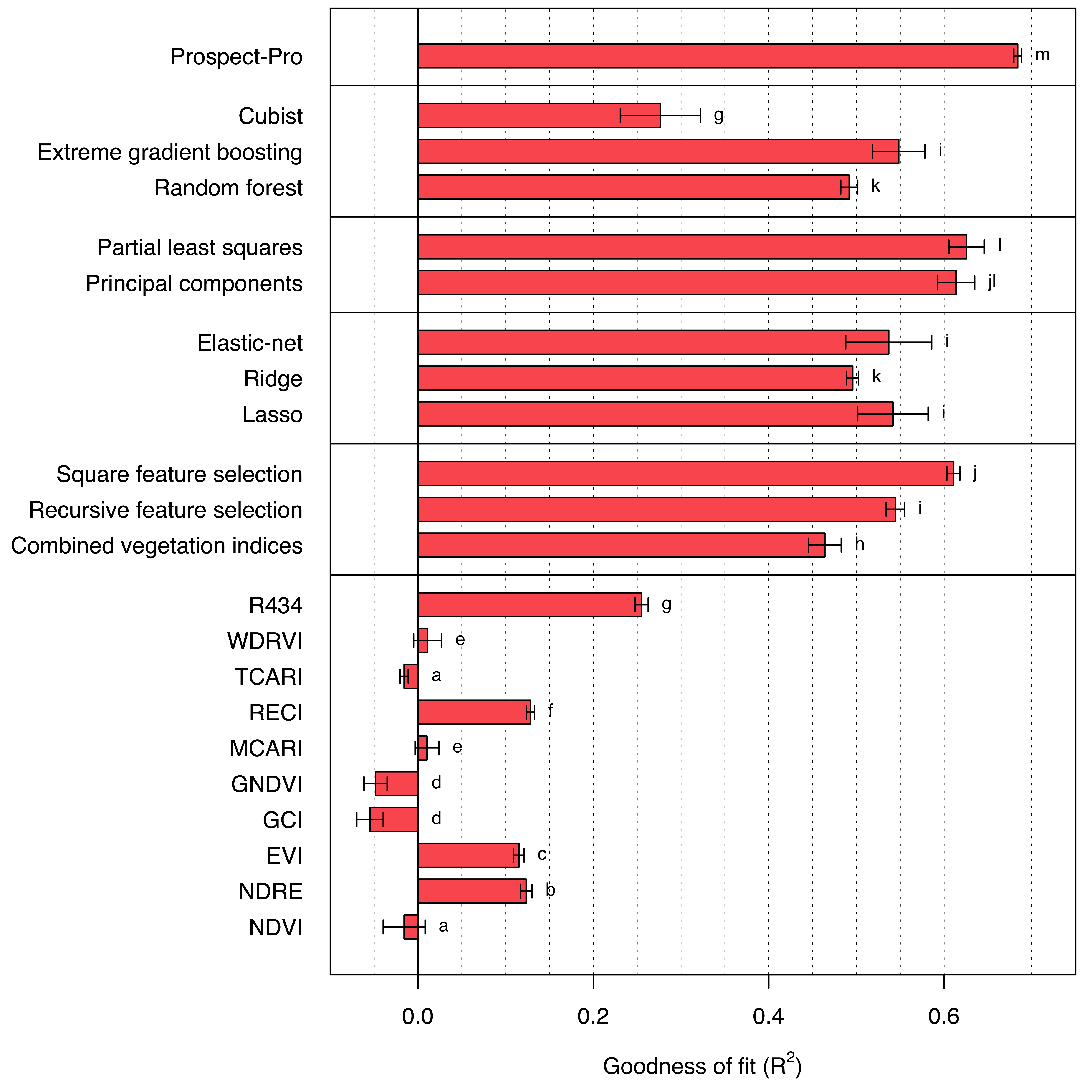
Indeed, Prospect-Pro achieves the best results in predicting area-based nitrogen content with a significant margin (R² = 0.684). The next best model, the partial least squares regression model, trails Prospect-Pro by 5.8 percentage points (R² = 0.626). Most of the implemented machine learning algorithms exceed an R² of 0.5, with the exception of cubist trees (Figure 7.1).

Interestingly, the square feature selection algorithm, which is relatively simple to implement, almost keeps pace with the best-performing machine learning methods (R² = 0.610). Single vegetation indices, on the other hand, do not correlate as well with area-based nitrogen. A single exception is the R434 which is the only vegetation index that utilizes information from blue bands (R² = 0.255). When combined, vegetation indices perform better, but this approach still falls short compared to most of the machine learning algorithms.

Mass-based nitrogen

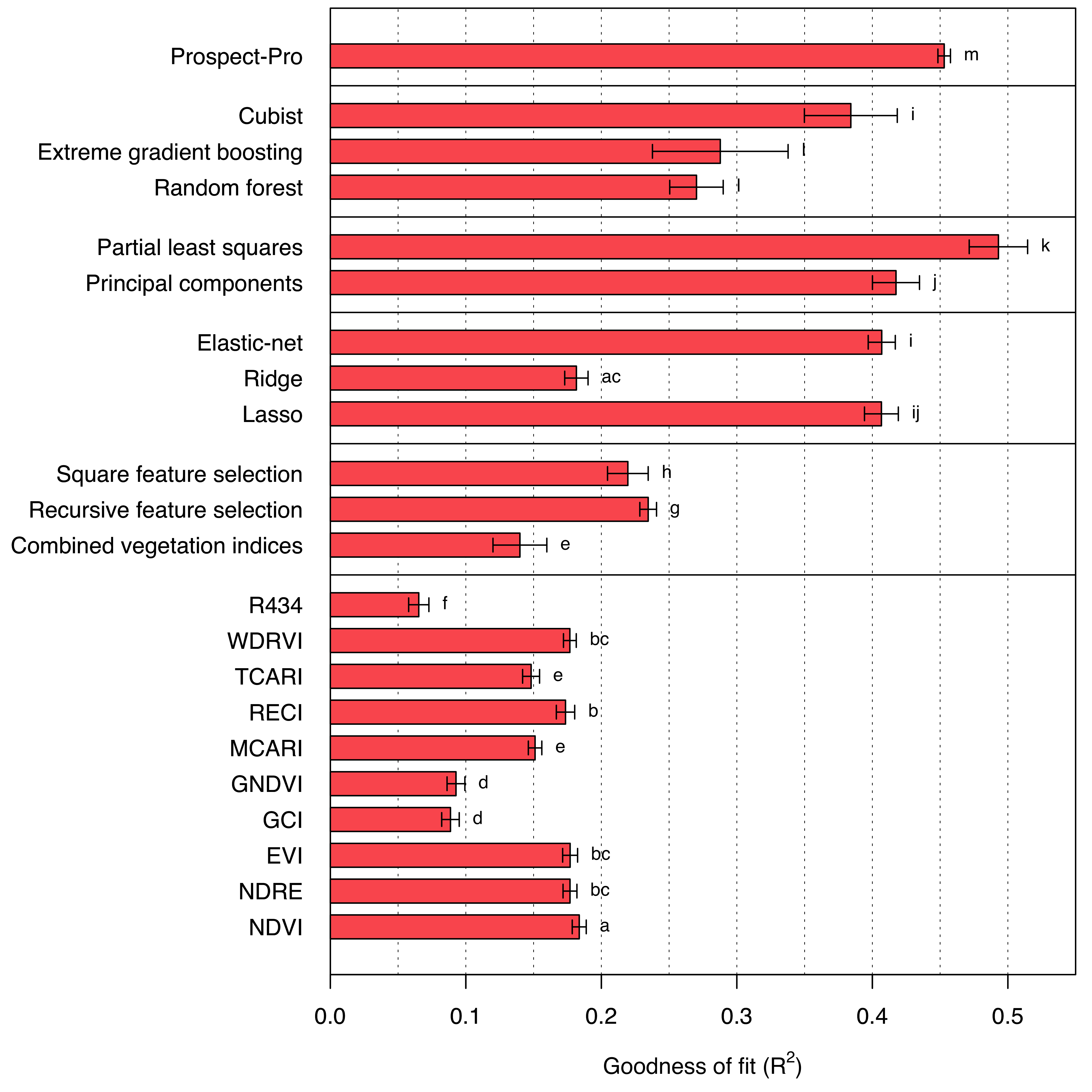
Shifting from area-based nitrogen to mass-based nitrogen, the predictive capability of previously leading models generally declines (Figure 7.2). Prospect-Pro still achieves relatively good results (R² = 0.453), but is outperformed by one of the machine learning models: the partial least squares regression model (R² = 0.493). Regrettably, estimating leaf mass per area from Prospect-Pro and using this estimation to convert units yielded worse results than directly applying a multiple linear regression model to the estimated (area-based) retrieved parameters. Meanwhile, directly using leaf mass per area to convert the retrieved parameters would have given the Prospect-Pro an unjust advantage over the machine learning models. However, the promising results of partial least squares regression suggest some potential for improvement in Prospect-Pro (or any related physics-based model) to predict the pigment concentrations.

Interestingly, the performance of ridge regression for mass-based nitrogen concentration drops much more than that of lasso regression, although ridge performed slightly worse than lasso on area-based nitrogen as well. Unlike ridge regression, which only shrinks linear model coefficients but never sets them to zero, lasso regression does precisely that: it sets the least important coefficients to zero, effectively leading to variable selection (James et al. 2013). Hence, if lasso regression outperforms ridge regression, this hints to the existence of a small number of relevant bands, while others can be disregarded.

The R434 vegetation index, which performed best for area-based nitrogen, fares the worst for mass-based nitrogen. Conversely, all vegetation indices that performed worse than the baseline model \(f(\mathbf x) = \bar y\) for area-based nitrogen significantly improved in the case of mass-based nitrogen. It is worth noting that vegetation indices, compared to other methods, exclusively utilize reflectance data. A possible explanation for their shortcomings in predicting area-based nitrogen is the correlation between transmittance and leaf mass per area, and subsequently any area-based trait.

Lastly, examining the standard deviation of cross-validated results reveals that the machine learning models in particular have very unstable outcomes (for both area-based and mass-based nitrogen), while Prospect-Pro prediction results appear to be comparatively stable. This can be attributed to the effective degrees of freedom of the models, which is much lower for physics-based models than for any machine-learning model, since there are only a few parameters to be estimated from the data.

7.2 Performance on the canopy level

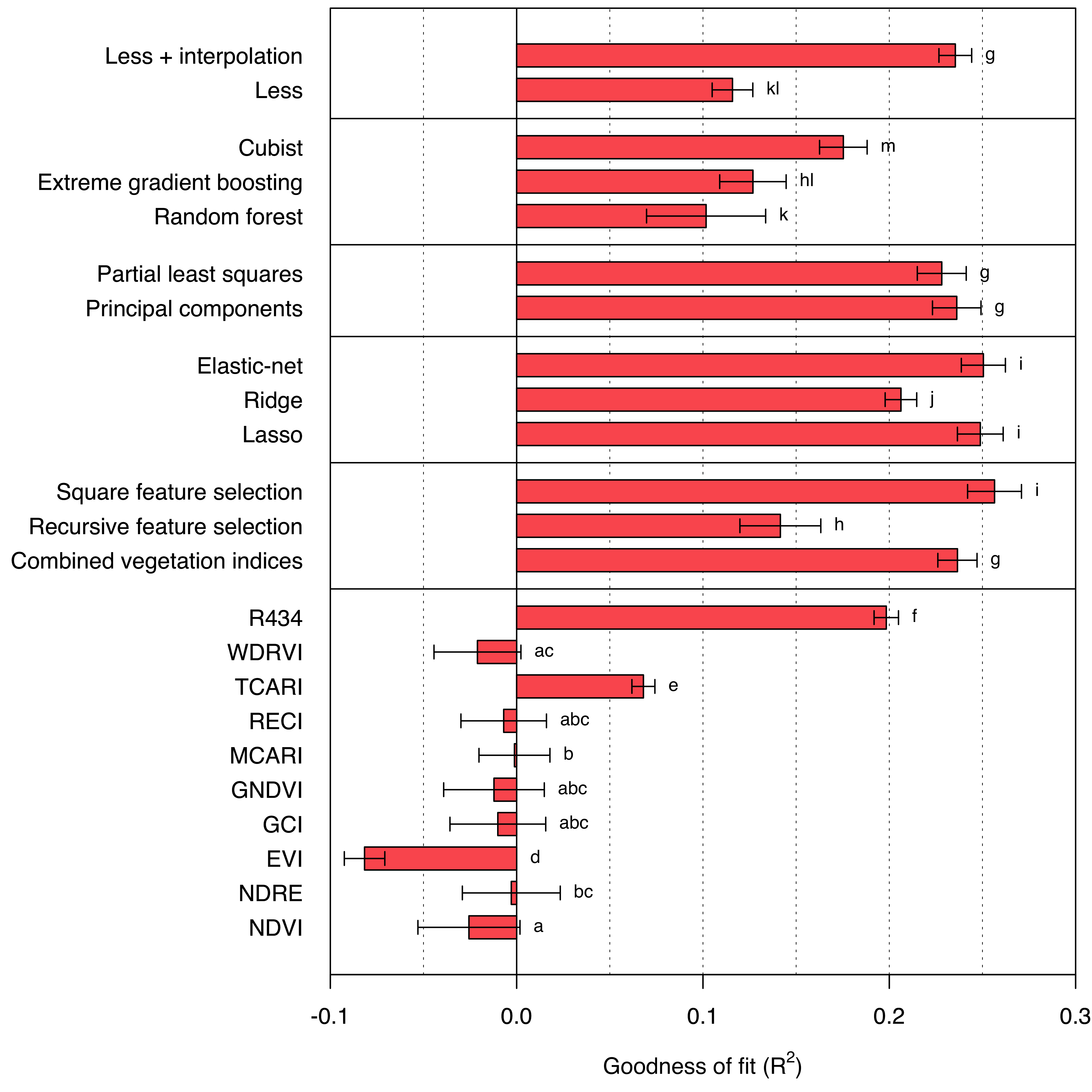
Focusing on the model performance results at the canopy level, the overall performance significantly declines compared to the leaf level (Figure 7.3). At best, the models appear to explain only 26% of the variance in the measured foliar nitrogen concentration. In this context, dimensionality reduction techniques slightly underperform compared to both lasso regression and elastic-net (R² = 0.249 and R² = 0.250, respectively). The gap between the elastic-net and ridge regression (R² = 0.206) is especially intriguing, considering the mixing parameter (\(\alpha = 0.1\)): the elastic-net coefficient penalization is a blend of 90% \(\ell^2\)-norm and only 10% \(\ell^1\)-norm (Table 6.2). Therefore, it leans heavily towards the penalization applied in ridge regression. However, the ability to completely eliminate coefficients appears to be highly beneficial. This outcome serves as an excellent illustration of the sensitivity of many machine learning models to minor alterations in their hyperparameters.

Figure 7.3: Performance of the different modelling methods in predicting the mass-based nitrogen (N_%) on a canopy-level. The value of the performance metric R² was calculated based on a 50 times repeated 20-fold cross-validation, of which the mean (\(\mu\)) and the standard deviation (\(\sigma\)) are reported. The compact letter display (CLD) next to every bar is derived from a pairwise Wilcoxon rank sum tests. Exact numerical values of the results can be found in the appendix in table 4.

One of the most striking outcomes is the substantial difference the hyper-dimensional interpolation has on the Less look-up table predictions. When the look-up table is used directly for predictions, the results are underwhelming (R² = 0.116). However, applying a surrogate model to achieve hyper-dimensional interpolation more than doubles the model performance (R² = 0.235). Consequently, by implementing the interpolation, the results produced by Less become comparable to machine-learning methods, despite the relatively low resolution of certain parameters in the look-up table.

Ironically, the best-performing model at the canopy level is not the widely praised partial least squares regression model, but rather the combination of square feature selection and the widely criticized stepwise selection (R² = 0.256).

In contrast to most other tested methods, vegetation indices perform rather poorly when applied to canopy-level data. Out of ten assessed vegetation indices, only two (TCARI and R434) manage outperform the baseline model \(f(\mathbf x) = \bar y\). Notably, the R434 vegetation index, introduced by Tian et al. (2011), is almost on par with the other more complex methods (R² = 0.198). It is the only vegetation index that utilizes information from blue bands (as to be seen in table 2.1).