Remote Sensing of Foliar Nitrogen in Californian Almonds

Master thesis presentation

Damian Oswald

damoswa@student.ethz.ch

April 11, 2024

Table of contents

• Background
• Explanation of the data
• Leaf-level radiative transfer modelling
• Canopy-level radiative transfer modelling
• Results of the model performances
• Discussion

Background

Almonds and nitrogen

• California is the largest producer of almonds with a production share of roughly 80% (CDFA 2020).

• Almonds are a profitable but also intensive crop, where the recommended nitrogen application ranges between 130 and 285 kg N ha^-1 a^-1 (Brown et al. 2020).

• Nitrogen leaching negatively impacts ecological systems and can affect the water supply quality (Yang et al. 2008).

• Remote sensing of crop nitrogen for an adequate fertilization is one of the core promises of precision agriculture (Walter et al. 2017).

Goal of this thesis

• Model the foliar nitrogen concentration based on hyperspectral images or spectroradiometric measurements.

\[ f: \boldsymbol \rho \in \mathbb R^{d} \longrightarrow \text{N}_{\%} \in \mathbb R \tag{1}\]

• Produce a model that is generalizable to datasets from other orchards and other years (and possibly even other crops).

Modelling approaches

I was trying out different modelling approaches to predict foliar nitrogen concentration from spectral data.

• Hand-crafted features (e.g. vegetation indices).

• Machine learning (purely data-driven).

• Modelling physical processes using radiative transfer models.

For this presentation, the focus will heavily lie on radiative transfer models.

Explanation of the data

Location of the almond orchard

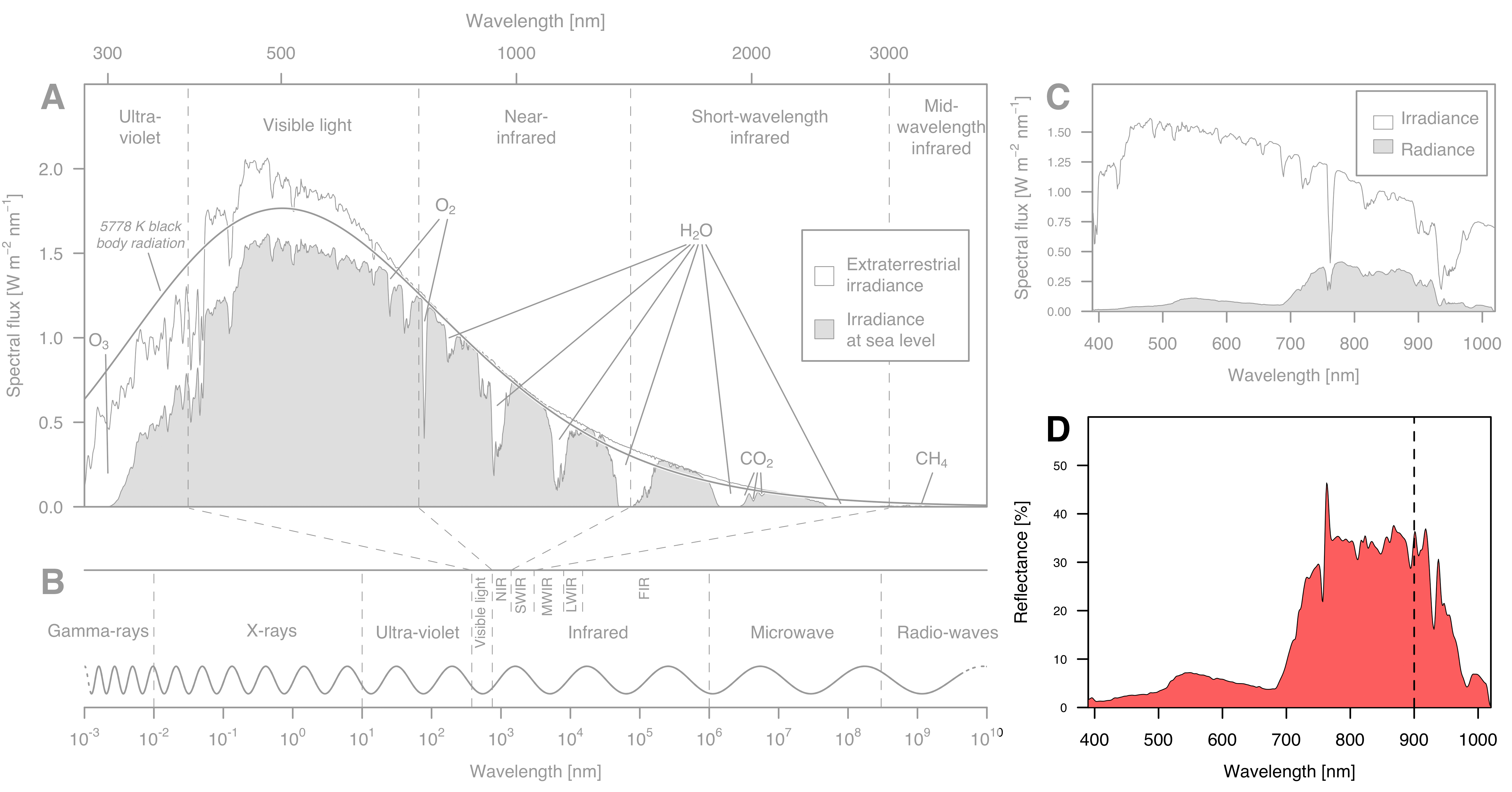
Hyperspectral data

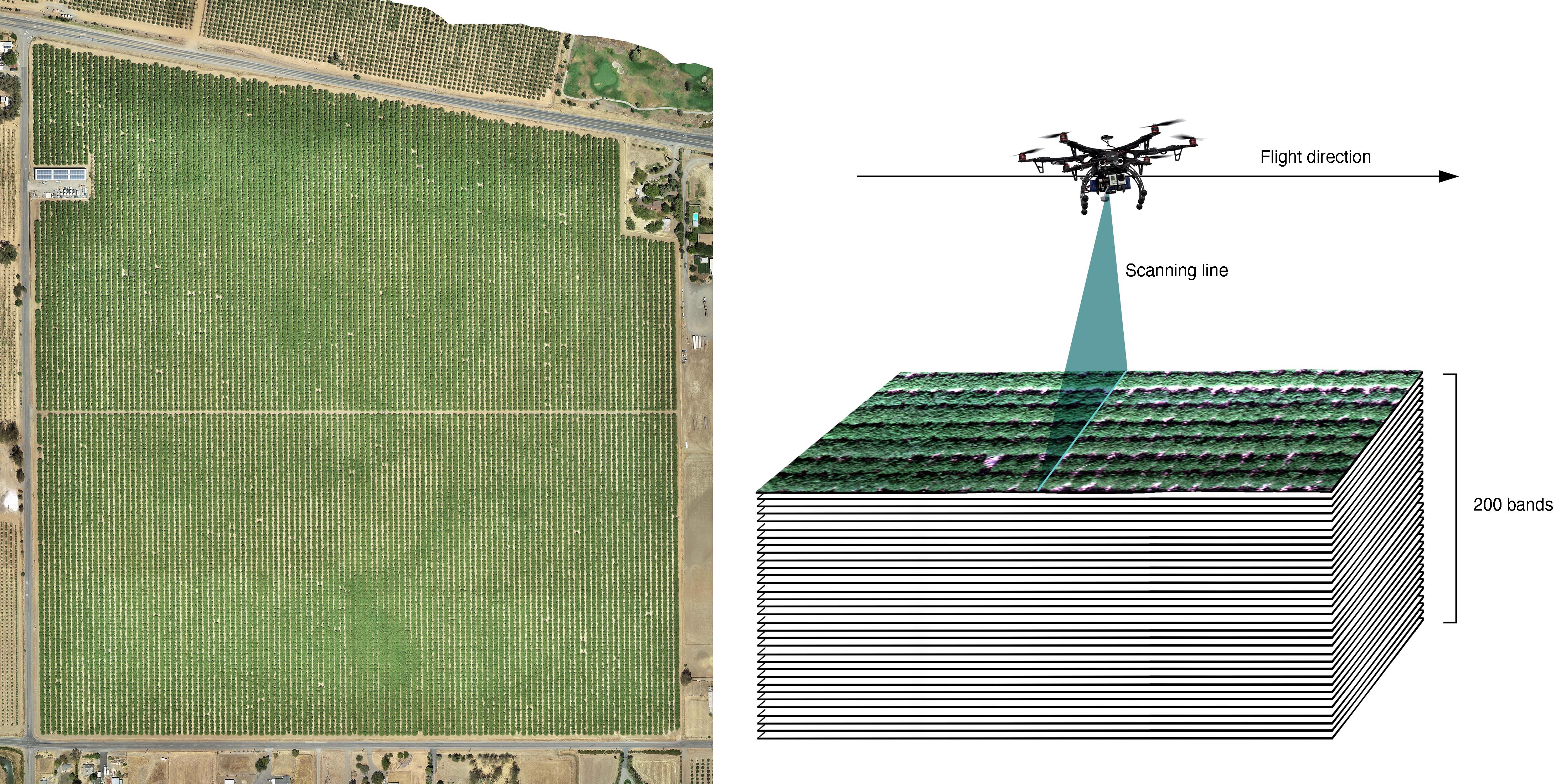
Figure 1: Westwind almond orchard in Woodland, CA (left). Explanation of hyperspectral images (right).

Pre-processing of the data

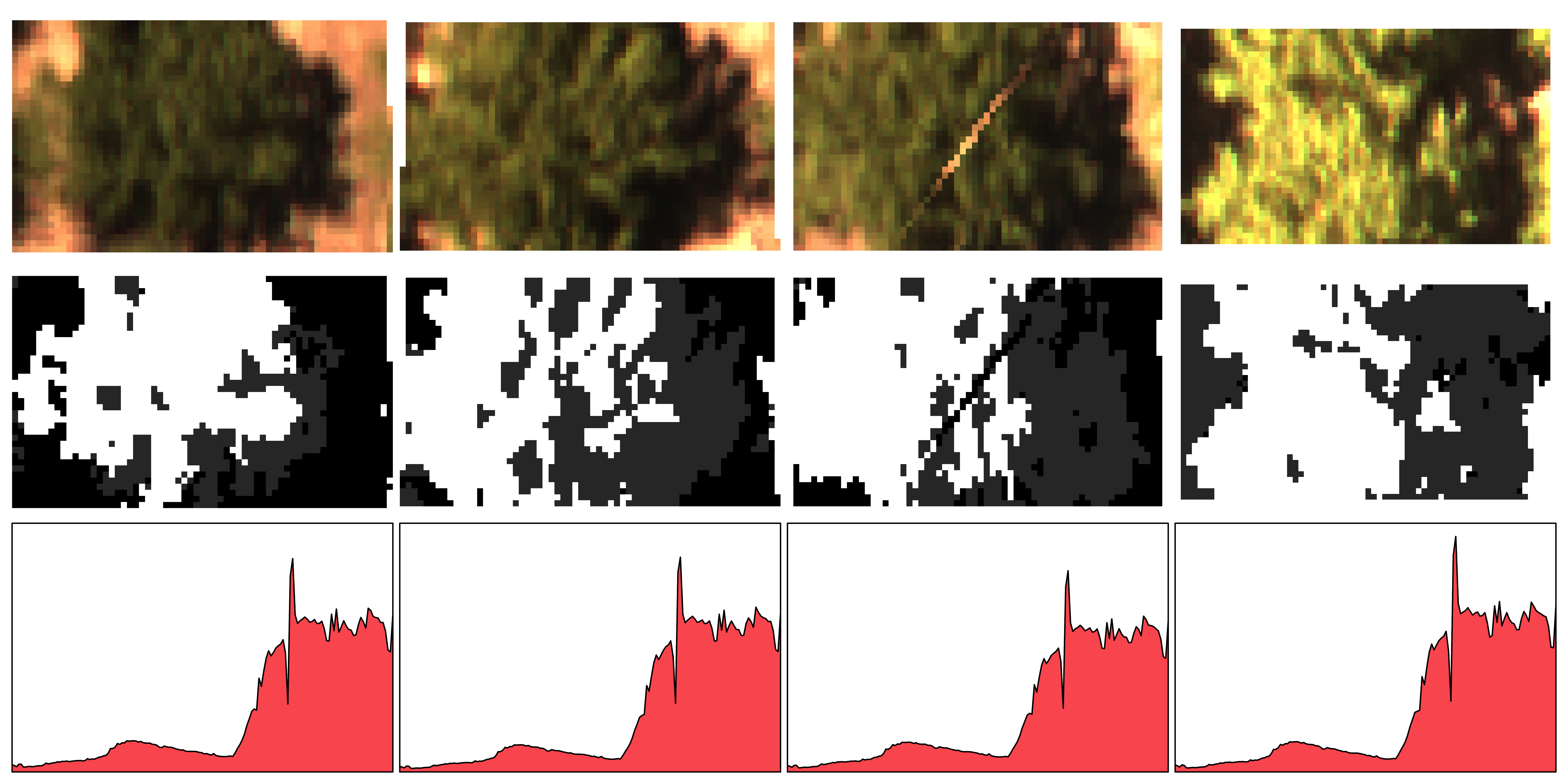
Figure 2: Segmentation process to extract the mean spectral reflectance from the hyperspectral images.

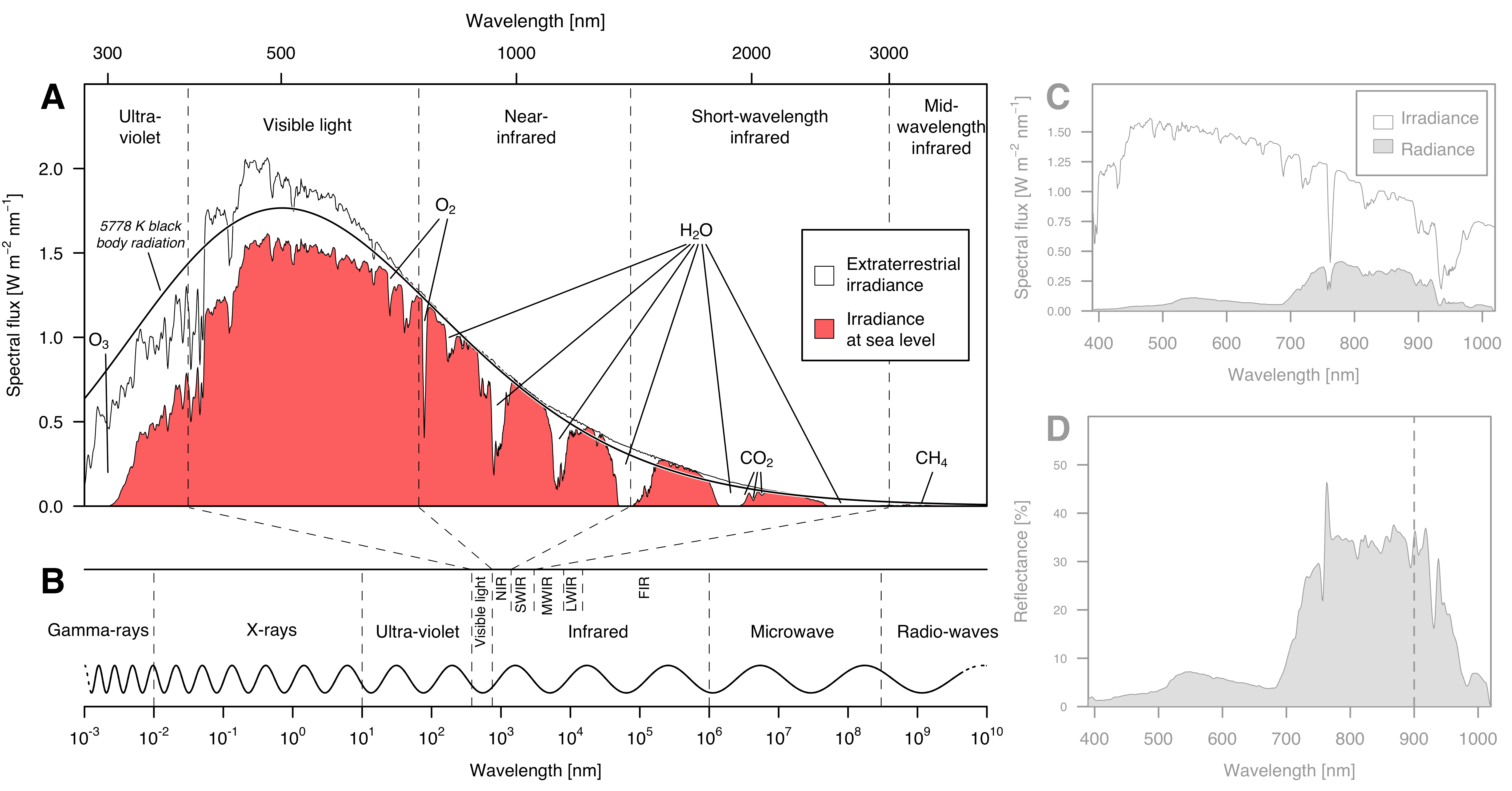
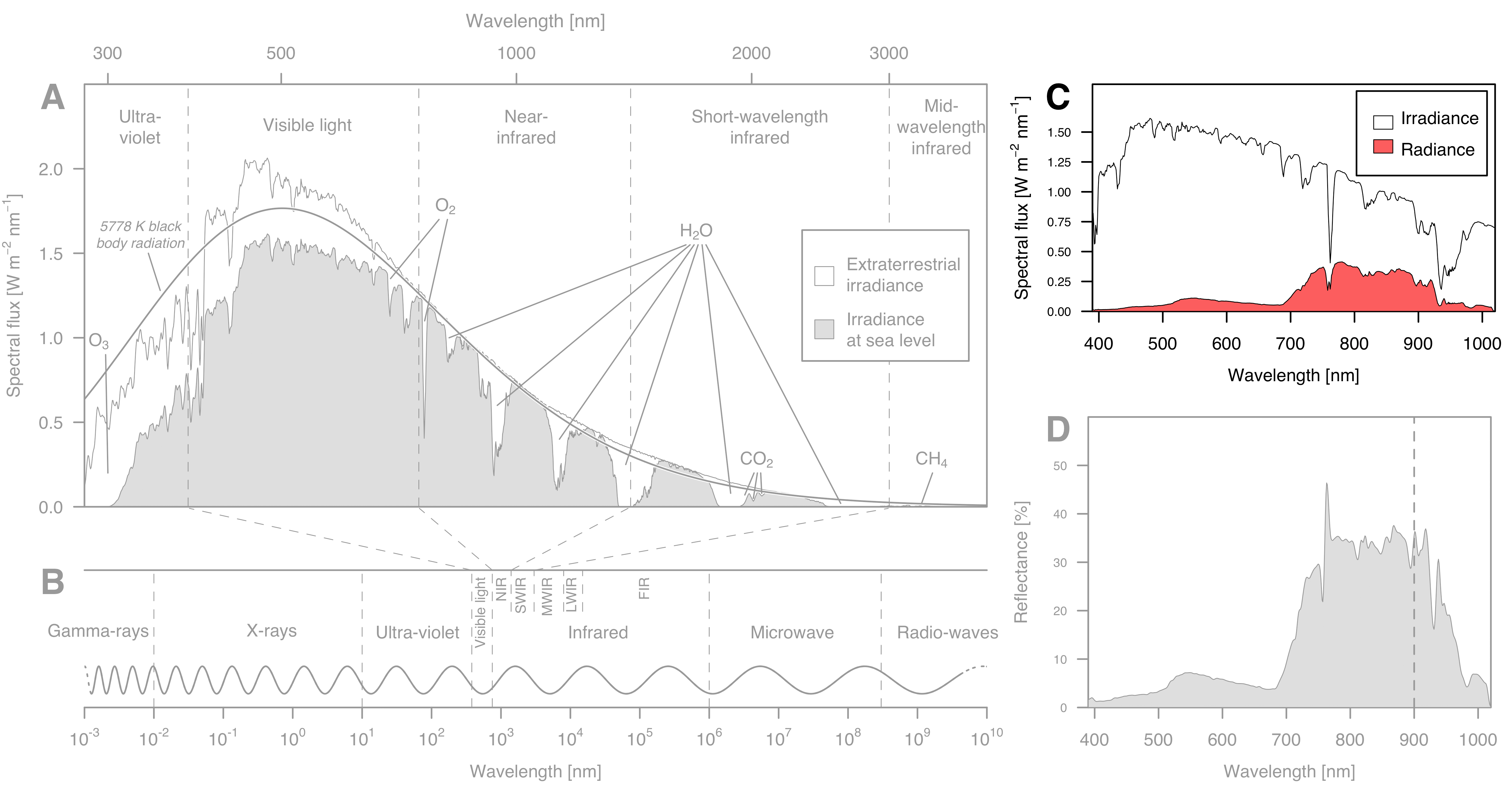
Irradiance, radiance, and reflectance

Overview of the data sets

Leaf-level and canopy-level data was used for this thesis, both referring to the same target trees.

Table 1: Overview of the two datasets used.

Level	Observations	Bands	Range	Sensor
Leaf	124	1024	338 - 2512 nm	HR-1024i
Canopy	107	151	385 - 900 nm	Pika L

Leaf-level radiative transfer modelling

The Prospect model

• Prospect (leaf optical property spectra) is a radiative transfer model first introduced by Jacquemoud (1992).

• It simulates the reflectance and transmittance of a leaf given the content of plant pigments (and some other plant parameters). \[ f: [\mathbf c, N, \alpha] \in \mathbb R^{9} \rightarrow [\boldsymbol \rho, \boldsymbol \tau] \in \mathbb R^{2\times 2101} \tag{2}\]

• The function \(f\) is constructed from established laws of physics.

The parameters of Prospect

Table 2: Input variables of the Prospect model as documented by Feret and de Boissieu (2022).

Abbreviation		Parameter	Unit
\(\mathbf c\)	CHL CAR ANT BROWN EWT PROT CBC	Chlorophyll content Carotenoid content Anthocyanin content Tannin content Equivalent water thickness Protein content Carbon-based constituent content	\(\mu \text{g cm}^{-2}\) \(\mu \text{g cm}^{-2}\) \(\mu \text{g cm}^{-2}\) \(-\) \(\text{g cm}^{-2}\) \(\text{g cm}^{-2}\) \(\text{g cm}^{-2}\)
\(N\)	N	Leaf mesophyll structure parameter
\(\alpha\)	alpha	Solid angle for incident light at surface of leaf	\(^{\circ}\)

Physics behind Prospect

We start out with equations describing s- and p-polarized transmission and reflection by Fresnel (1821), where \(n\) is the refractive index. \[ \scriptstyle t_s(\theta, n) = \frac{4\sqrt{1-\sin^2 \theta} \sqrt{n^2-\sin^2 \theta}}{\left(\sqrt{1-\sin^2 \theta} + \sqrt{n^2-\sin^2 \theta}\right)^2} \qquad t_p(\theta, n) = \frac{4n^2\sqrt{1-\sin^2 \theta} \sqrt{n^2-\sin^2 \theta}}{\left(n^2\sqrt{1-\sin^2 \theta} + \sqrt{n^2-\sin^2 \theta}\right)^2} \tag{3}\] We are interested in the transmissivity for diffuse light coming from all angles \(\theta\) between \(0\) and \(\frac{\pi}{2}\). \[ \scriptstyle \overline{T} = \frac{\int_0^{2\pi} d\varphi \int_0^{\alpha} t(\theta,n) \cos \theta \sin\theta d \theta}{\int_0^{2\pi} d\varphi \int_0^{\alpha} \cos \theta \sin\theta d \theta} \tag{4}\] The Fresnel equations were integrated by Allen (1973) for a general case of the maximum incidence angle \(\alpha\), both for s-polarized transmissivity:

\[ \scriptstyle \begin{aligned} T_s(\alpha, n) = \frac{1}{96}\frac{(n^2-1)^4}{\left[\sqrt{\left(\sin^2 \alpha -\frac{1}{2} (n^2 + 1)\right)^2 -\frac{1}{4} (n^2 - 1)^2} - \sin^2 \alpha +\frac{1}{2} (n^2 + 1)\right]^3} - \\\ \frac{1}{4}\frac{n^4 - 2n^2 +1}{\sqrt{\left(\sin^2 \alpha -\frac{1}{2} (n^2 + 1)\right)^2 -\frac{1}{4} (n^2 - 1)^2} - \sin^2 \alpha + \frac{1}{2} (n^2 + 1)} - \\\ \frac{1}{2} \left( \sqrt{\left(\sin^2 \alpha -\frac{1}{2} (n^2 + 1)\right)^2 -\frac{1}{4} (n^2 - 1)^2} - \sin^2 \alpha + \frac{1}{2} (n^2 + 1) \right) + \\\ \frac{1}{12} \frac{(n^2 - 1)^4}{(n + 1)^6} + \frac{1}{2} \frac{(n^2-1)^2}{(n+1)^2} + \frac{1}{4} (n^2+2n+1) \end{aligned} \tag{5}\]

As well as for p-polarized transmissivity:

\[ \scriptstyle \begin{aligned} T_p(\alpha, n) = \frac{-2 n^2}{(n^2 + 1)^2} \left[ \sqrt{\left(\sin^2 \alpha - \frac{1}{2} (n^2 + 1)\right)^2 - \frac{1}{4} (n^2 - 1)^2} - \sin^2 \alpha + \frac{1}{2} (n^2 + 1) - \frac{1}{2} (n + 1)^2 \right] - \\\ \frac{2 n^2 (n^2 + 1)}{(n^2-1)^2} \cdot \ln \left[ \sqrt{\left(\sin^2 \alpha - \frac{1}{2} (n^2 + 1)\right)^2 - \frac{1}{4} (n^2 - 1)^2} - \frac{\sin^2 \alpha - \frac{1}{2}(n^2 + 1)}{(n+1)^2} \right] + \\\ \frac{1}{2} n^2 \left\{ \left[ \sqrt{\left(\sin^2 \alpha - \frac{1}{2} (n^2 + 1)\right)^2 - \frac{1}{4} (n^2 - 1)^2} - \sin^2\alpha - \frac{1}{2} (n^2 + 1)\right]^{-1} - \frac{2}{(n + 1)^2} \right\} + \\ \frac{16n^4 (n^4 + 1)}{(n^2+1)^3(n^2-1)^2} \cdot \ln \left[\frac{ 2 (n^2 + 1) \left(\sqrt{\left(\sin^2 \alpha - \frac{1}{2} (n^2 + 1)\right)^2} - \sin^2 \alpha + \frac{1}{2} (n^2 + 1)\right) - (n^2 - 1)^2}{(n^2 + 1)(n + 1)^2 - (n^2-1)^2} \right] + \\\ \frac{16 n^6}{(n^2 + 1)^3} \left[ {2 (n^2 + 1) \left(\sqrt{\left(\sin^2 \alpha - \frac{1}{2} (n^2 + 1)\right)^2} - \sin^2 \alpha + \frac{1}{2} (n^2 + 1)\right) - (n^2 - 1)^2} \right]^{-1} - \\\ \frac{16n^6}{(n^2 + 1)^3\left( (n^2 + 1) (n + 1)^2 - (n^2 - 1)^2 \right)} \end{aligned} \tag{6}\]

Combine the two above to get the average transmissivity \(\overline{T}\) as a function of \(\alpha\) and \(n\).

\[ \scriptstyle \overline{T}(\alpha, n) = \frac{T_s(\alpha, n) + T_p(\alpha, n)}{2 \cdot \sin^2 \alpha} \tag{7}\]

The overall absorption coefficients \(k\) of a wavelength \(\lambda\) can be calculated as a weighted sum of specific absorption coefficients \(s\), where the weights are the content of the plant pigments. These specific absorption coefficients were empirically estimated by Féret et al. (2021).

\[ \scriptstyle k_\lambda = \frac{1}{N} \sum_i c_i s_{i,\lambda} \tag{8}\]

Given this coefficient vector, we can calculate the transmission for isotropic light \(\varphi\) for every wavelength \(\lambda\) with \(k = k_\lambda\) using the upper incomplete gamma function according to the Beer-Lambert law (Lambert 1760; Beer 1852).

\[ \scriptstyle \varphi = (1 - k) \cdot e^{-k} + k^2 \cdot \Gamma(k) = (1 - k) \cdot e^{-k} + k^2 \cdot \int_k^\infty \frac{e^{-t}}{t} dt \tag{9}\]

Given all of the equations above, Jacquemoud (1992) wrote the first implementation of the Prospect model. \[ \scriptstyle \begin{aligned} A = \frac{ \varphi \: \overline T(90, n)} { n^2\left[1 - \varphi^2 \: \left(1 - n^{-2} \: \overline T(90, n) \right)^2\right] } \qquad B = \overline T(90, n) \: A \\[15pt] C = 1 - \overline T(90, n) + \varphi \: B \: \left(1 - \frac{\overline T(90, n)}{n^2}\right) \\[15pt] D = \sqrt{(1 + C + B) \: (1 + C - B) \: (1 - C + B) \: (1 - C - B)} \qquad E = \frac{1 + C^2 - B^2 + D}{2\,C} \\[15pt] F = \frac{1 - C^2 + B^2 + D}{2\,B} \qquad G = F^{N-1} \qquad H = \frac{E \, (G^2 - 1)}{E^2 \, G^2 - 1} \end{aligned} \tag{10}\] Everything can be put together to get the spectral reflectance \(\rho\) and transmittance \(\tau\) of a leaf. \[ \scriptstyle \rho = 1 - \overline T(\alpha, n) \left[ 1 + \varphi \, A \left(1 - \frac{\overline T(90, n)}{n^2} \right) + \frac{A \, H \, B}{1 - H \, C} \right] \tag{11}\] \[ \scriptstyle \tau = \frac{\overline T(\alpha, n) \, A \, G \, (E^2 - 1)}{(E^2 \, G^2 - 1) \, (1 - H \, C)} \tag{12}\]

Interactive demonstration

The inversion problem

• Radiative transfer models are constructed in the forward mode: we calculate the reflectance given leaf parameters.

• In reality, we are dealing with the inverse problem: we already know the reflectance, but want to find the parameters. This is called the backward mode. \[ f: x \to y \qquad \qquad f^{-1}: y \to x \tag{13}\]

• The inversion can be achieved via (1) optimization, (2) a look-up table or (3) machine learning.

Canopy-level radiative transfer modelling

The Less model

• The Less model (large-scale emulation system for forest simulation) is a ray tracing model developed by Qi et al. (2019).

• It simulates a three-dimensional scene given the spectral reflectance of every material used.

• Less is computationally much more intensive than Prospect and also includes many more parameters.

• The inversion of Less was achieved using a look-up table.

Modelling the orchard scene

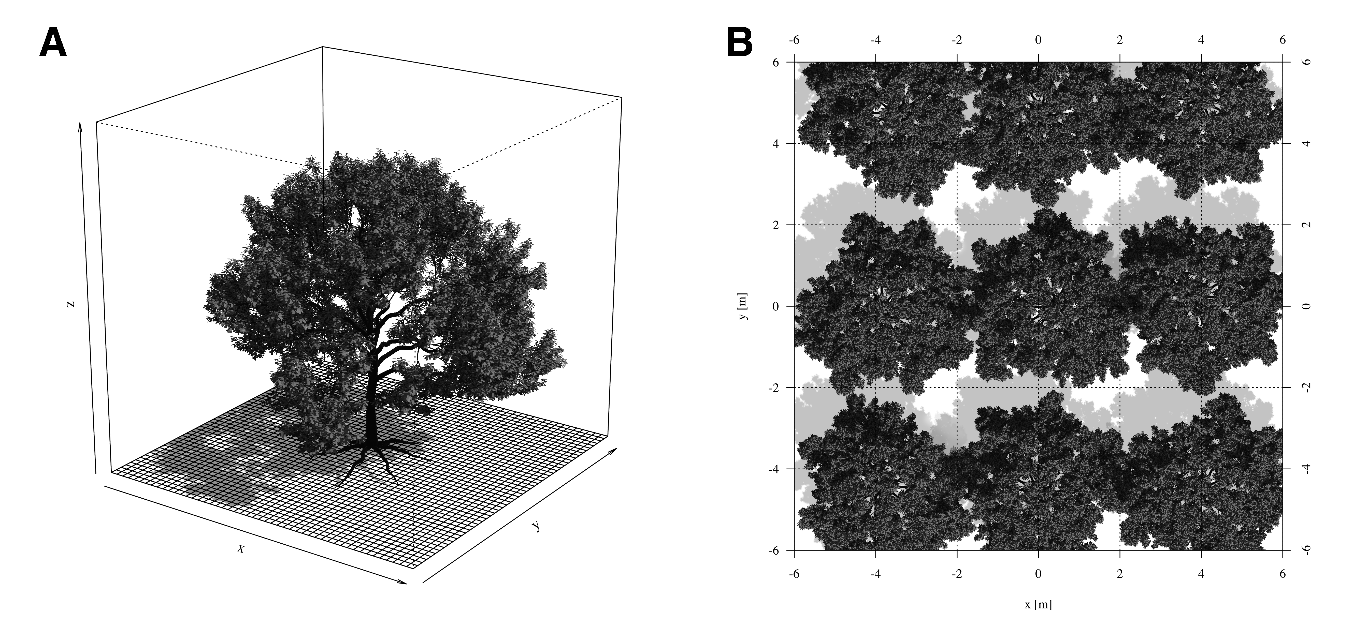
Figure 3: The preliminarily used three-dimensional model of an almond tree (A) and how it is arranged to represent a tree in the orchard (B).

Observation vs. simulation

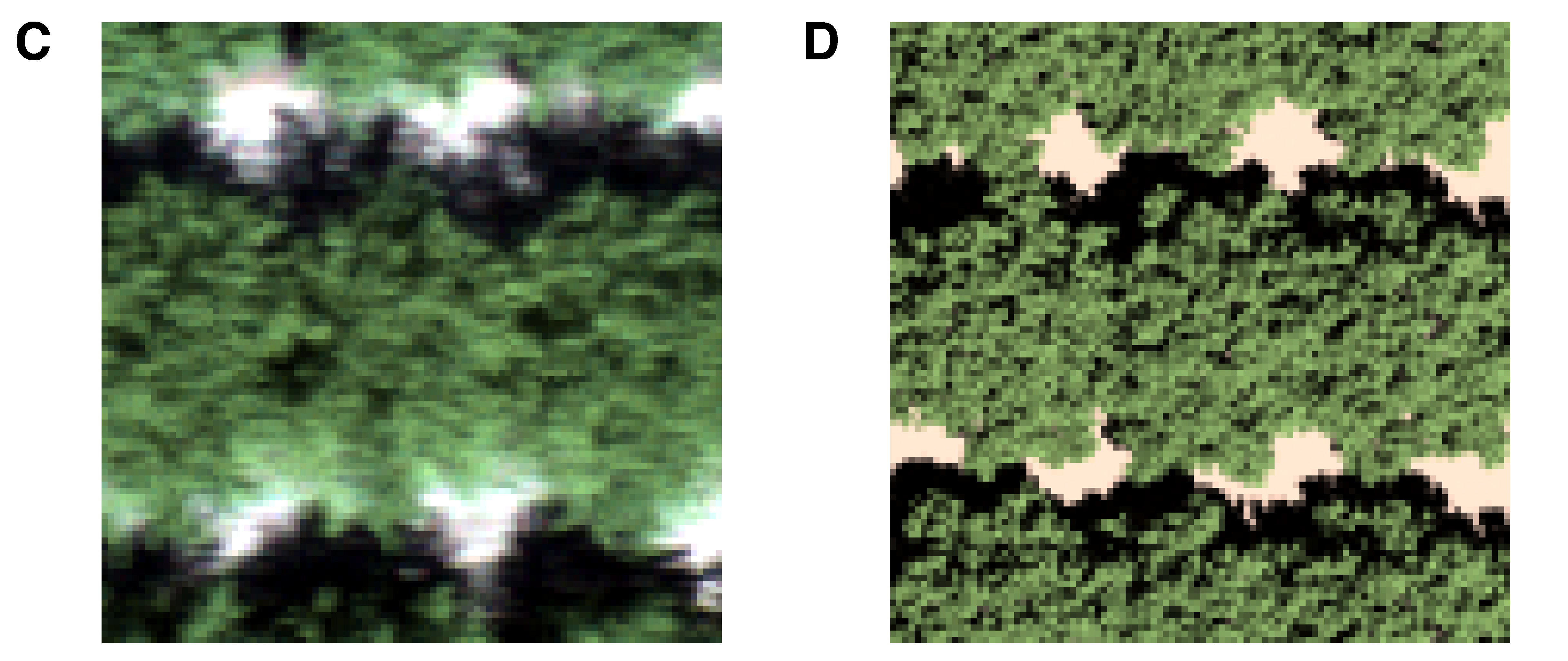
Figure 4: An RGB representation of the hyperspectral data which was observed (C) compared to the one that was simulated (D).

Look-up-table regression

• Generated a look-up table containing 16’500 simulations.

• Given one observation, we find its closest match in the look-up table by minimizing a cost function \(J\). \[ J = \frac{1}{d} \sum_{\lambda=1}^d w_i\left( \rho_{\lambda,\text{obs.}} - \rho_{\lambda,\text{sim.}} \right)^2 \tag{14}\]

• Make smooth predictions by applying hyper-dimensional interpolation (multicubic polynomial surrogate model).

Results of the model performances

Leaf level results (area-based N)

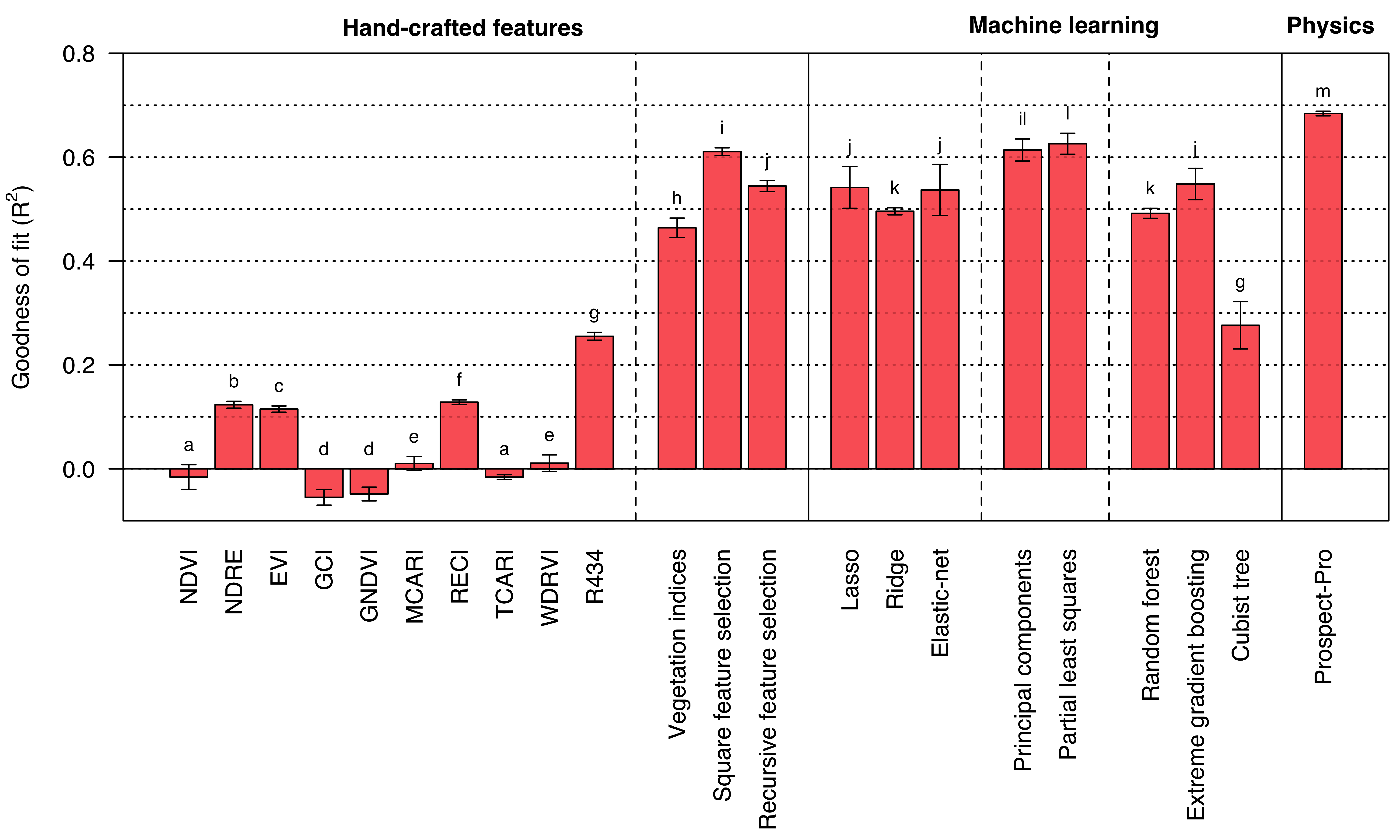
Figure 5: Results based on a 50 times repeated 20-fold cross validation.

Leaf level results (mass-based N)

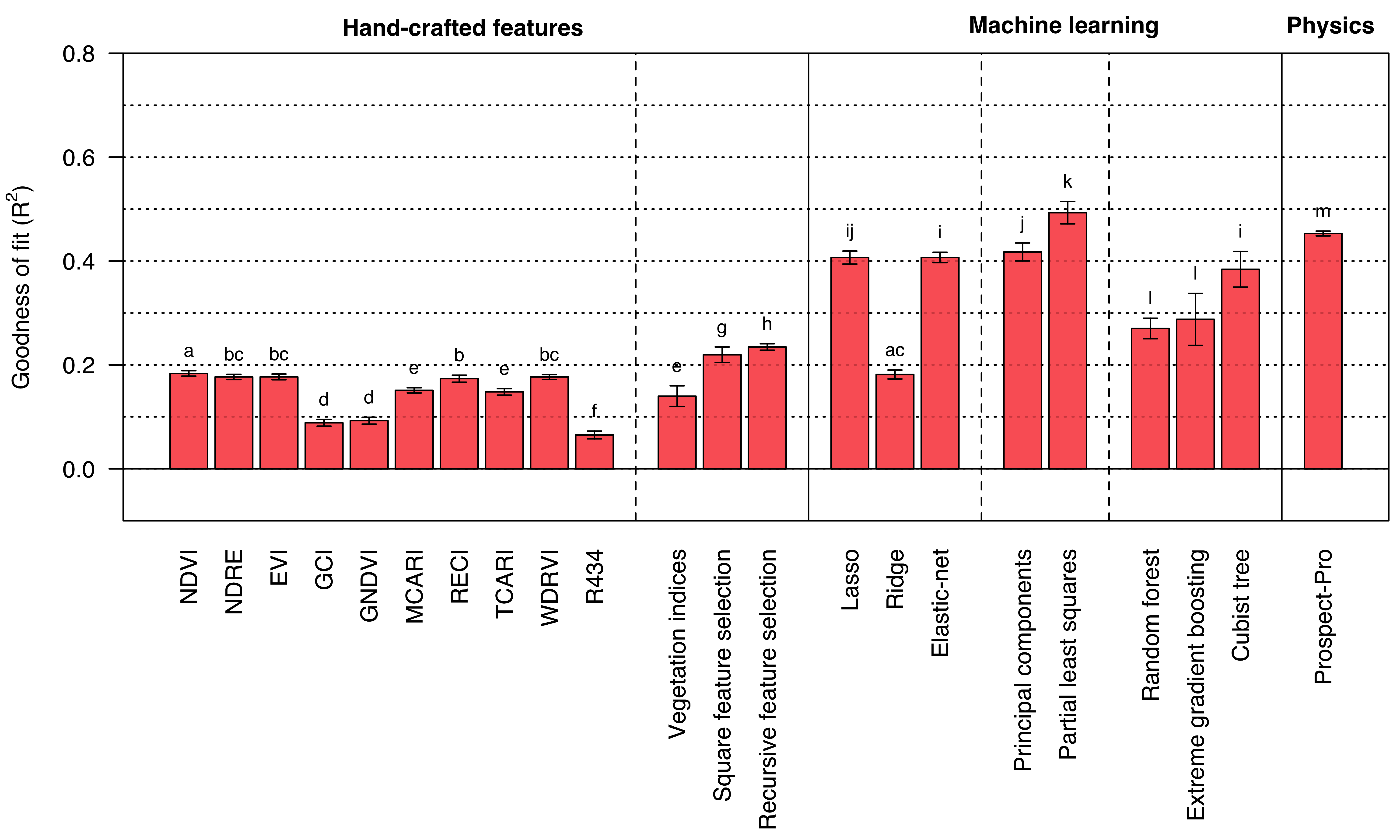
Figure 6: Results based on a 50 times repeated 20-fold cross validation.

Canopy level results

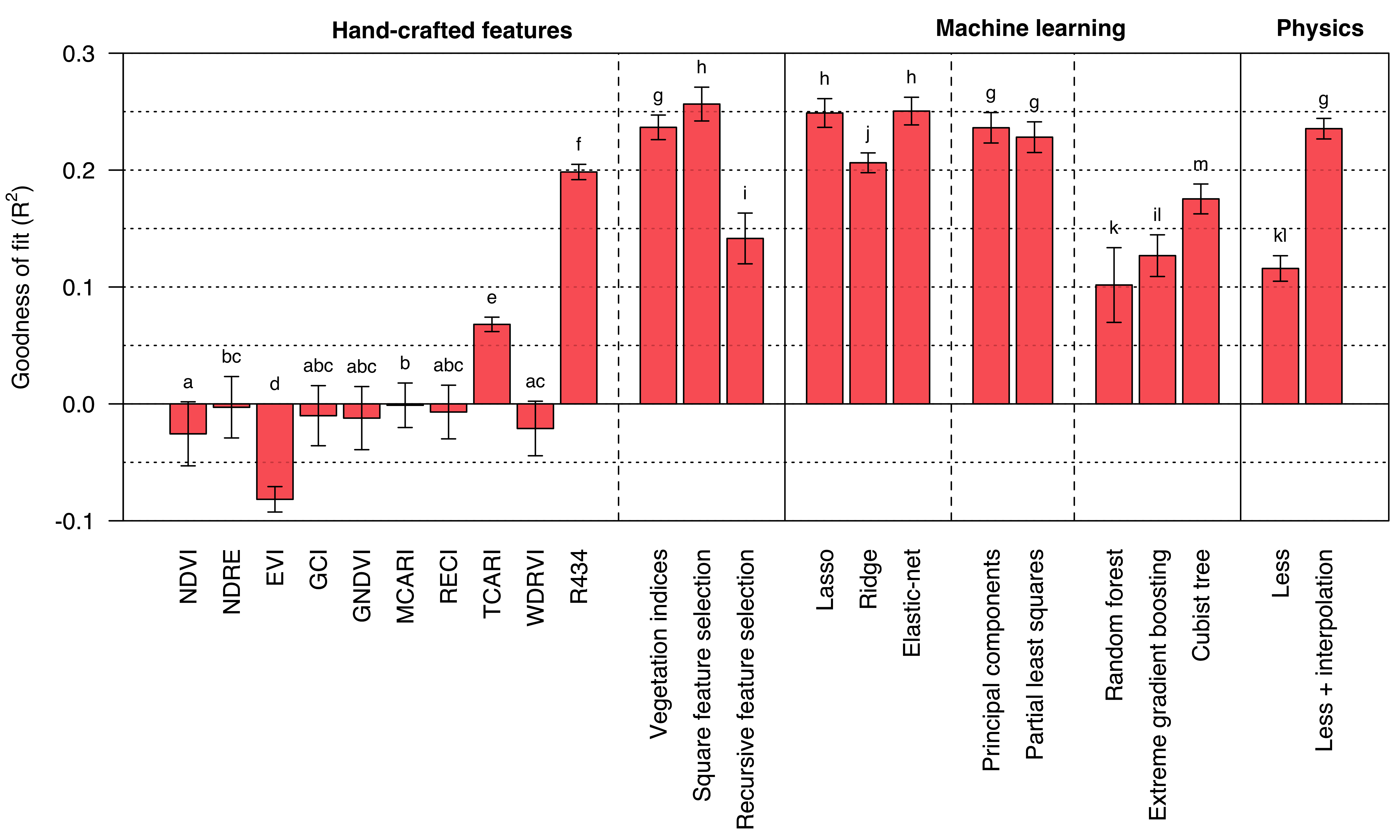
Figure 7: Results based on a 50 times repeated 20-fold cross validation.

Discussion

Machine learning or physics?

• Machine learning models work well, but they tend not to be robust if applied to settings outside their training data.

• Physics-based models may provide this robustness while maintaining a similar level of accuracy (Berger et al. 2018).

• These models also push the understanding of the subject more than machine learning models do.

• Machine learning serves well as an indicator of what level of accuracy should be expected.

Range of the nitrogen measurements

• Data set covers a commercial almond orchard fertilized according to the recommendations. The measured N_% ranges between 1.96 and 3.17%.

• Much of the published research focuses on fertilization trials, where nitrogen deficiency is artificially induced.

• Healthy distrust of nitrogen measurements – they are no absolute ground truth.

Improving canopy-level predictions

• Include information in the short-wave infrared spectrum from more advanced sensors.

• Spatial information can be combined with spectral information to predict foliar nitrogen concentrations.

Conclusion

• Nitrogen remote sensing research should focus on crops that are fertilized according to standard practice.

• Radiative transfer models are promising as a robust method of estimating plant traits which can be connected to N_%.

• Prospect predictions shows discrepancies with observed data: chlorophyll could be split into chlorophyll a and b.

• Spectral resolution is not that important – but the range covered is (especially short-wave infrared).

References

Allen, William A. 1973. “Transmission of Isotropic Light Across a Dielectric Surface in Two and Three Dimensions.” JOSA 63 (6): 664–66. https://doi.org/10.1364/JOSA.63.000664.

Beer, August. 1852. “Bestimmung Der Absorption Des Rothen Lichts in Farbigen Flussigkeiten.” Ann. Physik 162: 78–88.

Berger, Katja, Clement Atzberger, Martin Danner, Guido D’Urso, Wolfram Mauser, Francesco Vuolo, and Tobias Hank. 2018. “Evaluation of the PROSAIL Model Capabilities for Future Hyperspectral Model Environments: A Review Study.” Remote Sensing 10 (1): 85. https://doi.org/10.3390/rs10010085.

Brown, Patrick H., Sebastian Saa, Saiful Muhammad, and Sat Darshan Khalsa. 2020. “Nitrogen Best Management Practices.” 1150 Ninth Street, Suite 1500, Modesto, CA 95354: Almond Board of California.

CDFA. 2020. “California Agriculture Exports 2019-2020.” 1220 N Street, Sacramento, CA 95812: California Department of Food and Argiculture.

Feret, Jean-Baptiste, and Florian de Boissieu. 2022. Prospect: PROSPECT Leaf Radiative Transfer Model and Inversion Routines. https://gitlab.com/jbferet/prospect.

Féret, Jean-Baptiste, Katja Berger, Florian De Boissieu, and Zbyněk Malenovskỳ. 2021. “PROSPECT-PRO for Estimating Content of Nitrogen-Containing Leaf Proteins and Other Carbon-Based Constituents.” Remote Sensing of Environment 252: 112173. https://doi.org/10.1016/j.rse.2020.112173.

Fresnel, Augustin. 1821. “Note Sur Le Calcul Des Teintes Que La Polarisation développe Dans Leslames Cristallisées.” Annales de Chimie Et de Physique 17 (2): 102–11.

Jacquemoud, Stéphane. 1992. “Utilisation de La Haute Resolution Spectrale Pour l’etude Des Couverts Vegetaux: Developpement d’un Modele de Reflectance Spectrale.” PhD thesis, Université Paris Diderot-Paris 7.

Lambert, Johann Heinrich. 1760. Photometria Sive de Mensura Et Gradibus Luminis, Colorum Et Umbrae. Sumptibus vidvae E. Klett, typis CP Detleffsen.

Qi, Jianbo, Donghui Xie, Tiangang Yin, Guangjian Yan, Jean-Philippe Gastellu-Etchegorry, Linyuan Li, Wuming Zhang, Xihan Mu, and Leslie K Norford. 2019. “LESS: LargE-Scale Remote Sensing Data and Image Simulation Framework over Heterogeneous 3D Scenes.” Remote Sensing of Environment 221: 695–706. https://doi.org/10.1016/j.rse.2018.11.036.

Walter, Achim, Robert Finger, Robert Huber, and Nina Buchmann. 2017. “Smart Farming Is Key to Developing Sustainable Agriculture.” Proceedings of the National Academy of Sciences 114 (24): 6148–50. https://doi.org/10.1073/pnas.1707462114.

Yang, Xiao-e, Xiang Wu, Hu-lin Hao, and Zhen-li He. 2008. “Mechanisms and Assessment of Water Eutrophication.” Journal of Zhejiang University Science B 9 (3): 197–209. https://doi.org/10.1631/jzus.B0710626.